
NumPy and SciPy Eigen-Analysis and ODE Solutions for Gene Expression Models
Published:
Numerical and analytical work in Python, using NumPy, SciPy and Matplotlib, on the mathematics that underlies dynamic models of gene regulation.
Root finding, three ways
For sin squared x = 1 - x: a graphical estimate, a first-order Taylor expansion about pi/4, and SciPy’s brentq. All three land near 0.64, which is the reason to do all three. An analytical approximation and a numerical solver agreeing is the only cheap check either one gets.
An ODE model of gene expression
A model of expression saturating at p = 1, solved analytically, verified by plotting the solution against the numerical integration, and then averaged across the interval with scipy.integrate.quad.
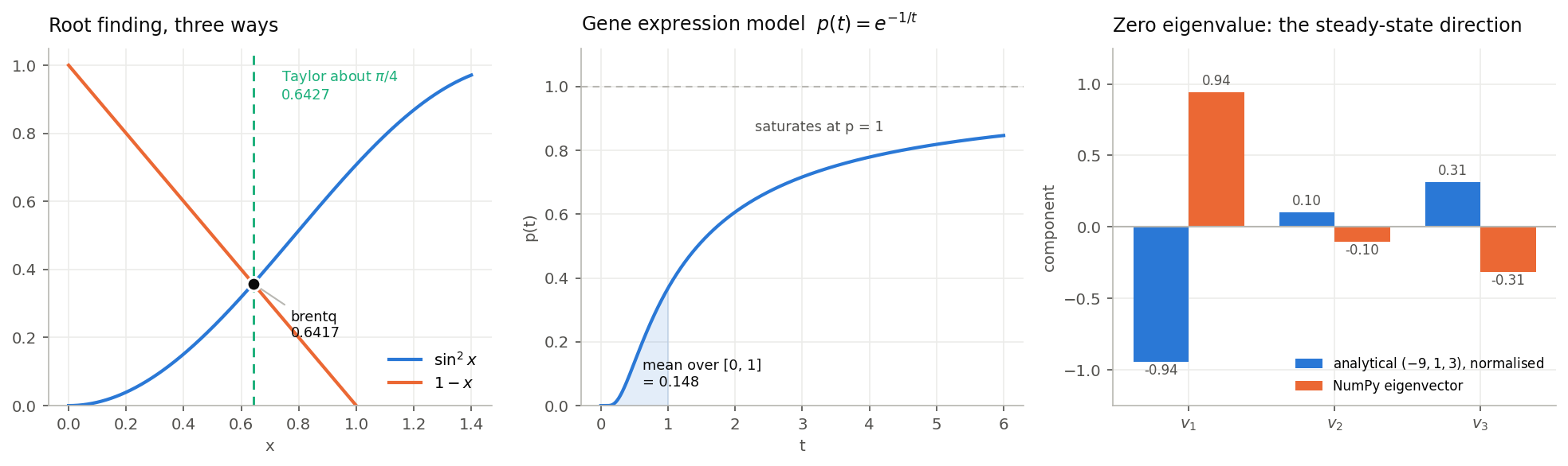
Left: the two curves meet once, and the graphical estimate, the Taylor expansion about pi/4 (0.6427) and brentq (0.6417) all land in the same place. Middle: the solution approaches 1 without reaching it, with the shaded interval whose mean the numerical integration returns as 0.148. Right: the eigenvector for the zero eigenvalue, where NumPy returns the analytical vector normalised and sign-flipped. That is not a disagreement, because an eigenvector is only defined up to scale.
Eigen-analysis of a linear system
A three-variable linear ODE system written in matrix form, with eigenvalues and eigenvectors derived by hand and then recomputed with NumPy, checked against solve_ivp.
The zero eigenvalue is the interesting one. It means a direction in which the system does not move at all, which is to say a steady state: the model conserves something. That is a structural property of the system, not a numerical artefact, and it is visible in the linear algebra before any trajectory is simulated.
Critiquing an LLM’s answers
Two parts of the assignment asked for a critique of ChatGPT’s solutions to the same problems. It chose an unnecessarily wide bracketing interval, defaulted to fsolve where a bracketing method was better suited, got the linearised root wrong, and explained the zero eigenvalue in generic textbook terms rather than for the system actually in front of it.